When Machine Learning Takes the Stand

Section I: A Ground-Up Explanation of Simple Machine Learning
To understand machine learning, I find it helpful to first break the process down into its simplest components. In this pursuit, I wrote the following hypothetical which outlines the creation of a machine learning algorithm from the ground up:
In suing a corporation for violations of the Telecommunication Consumer Protection Act (“TCPA”), a class action plaintiff’s attorney subpoenas the defendant corporation’s call records. The defendant-corporation produces thirty-million unique call records, each identifying: (1) the date of the call, (2) the individual who received the call, (3) the transcript of the call, and (4) whether the receiver of the call consented to the corporation’s contact.
The plaintiff’s attorney would like to review these records in order to discover additional class members, but, even at a rate of 1-second-per-record, reviewing the thirty-million records by hand would take him 8,333.33 hours. Accordingly, the attorney creates a program to review the records under the following parameters:
1. If [date of the call] is after the [the TCPA’s effective date], and
a. If the individual who received the call did not consent to the call, or
2. If the individual who received the call consented to the call—but thereafter reneged consent,
3. Then, the individual who received the call is a member of the injured class.
The program runs each record through these parameters and separates each into two groups: records of phone calls made in violation of the TCPA (thus containing class members) and records of non-violative phone calls. Using a standard computer, the attorney’s algorithm could process all thirty-million records in about 1/16th of a second. For purposes of this hypothetical, let’s say the resultant data initially tallies only 10,000 class-members to 29,990,000 non-class members. The attorney knows 10,000 is too low a number to be accurate, so he adds another condition to the algorithm:
1. If [date of the call] is after the [the TCPA’s effective date], and
a. If individual who received the call did not consent to the call, or
b. If individual who received the call consented to the call but thereafter reneged consent, or
c. If the transcript reveals the defendant’s employee violated the TCPA,
2. Then, the call violated the TCPA and the individual who received the call is a class member.
Now, in order for the algorithm to function, it needs some method of determining what about the contents of a transcript constitutes a TCPA violation. Appreciating the complexity of what constitutes a TCPA violation, the attorney likely cannot effectively list out each deciding datum. Instead, the attorney can imbue its algorithm with machine learning by coaching it to make these determinations on its own using the following method:
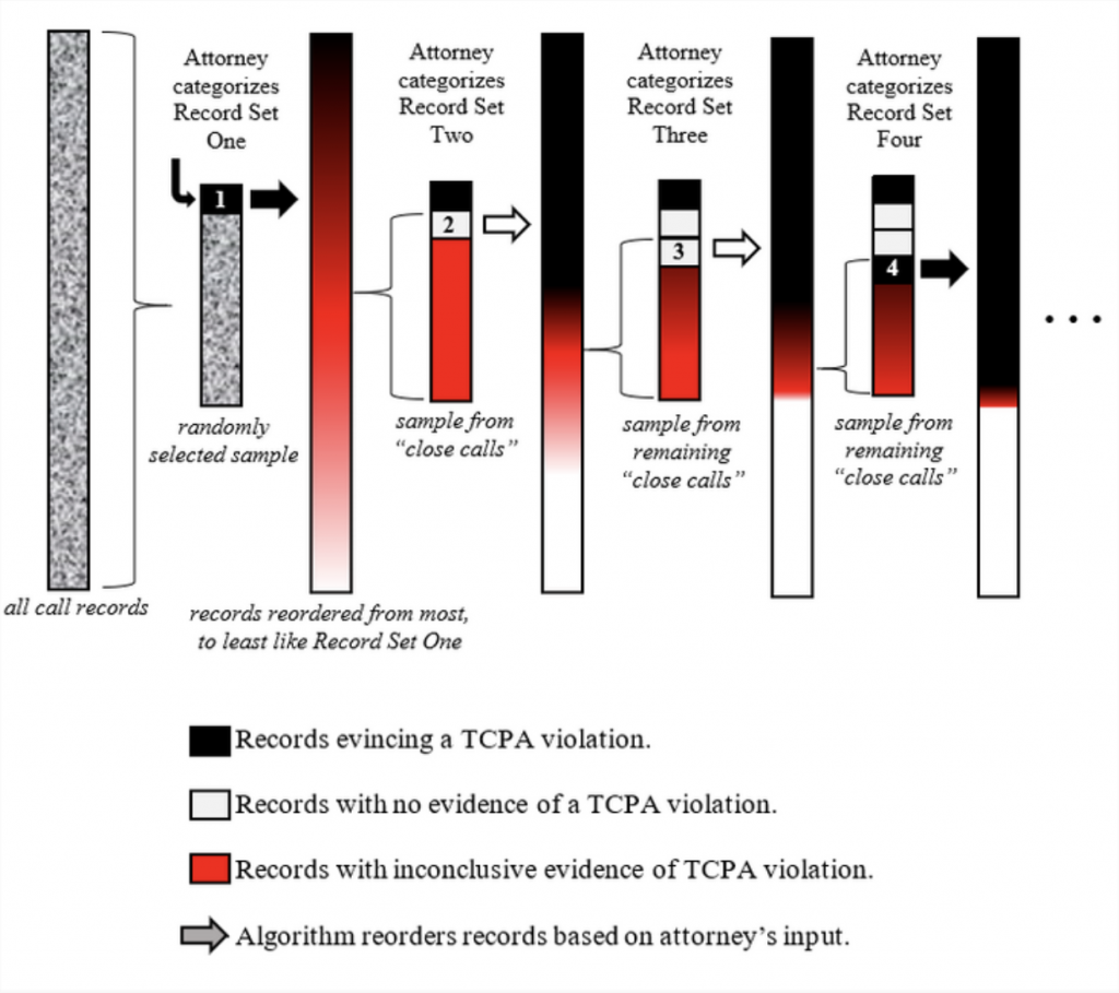
First, the attorney takes a randomly-selected sample of 10 call records from the 29,990,000 (“Record Set One”). He reviews one of those records and finds that the transcript of the call shows that the defendant’s employee failed to disclose that she was making a sales call, thereby violating the TCPA’s disclosure requirement. Accordingly, the attorney marks that as a “class member” record and moves onto the next randomly selected record in Record Set One. Once he’s reviewed each record in Record Set One, the algorithm compares those to the remaining 29,989,990 and reorders them according to each record’s degree of similarity to the records marked as “class member records” in Record Set One. Because the algorithm is basing this reorganization on only 10 categorized emails, the reorganized list is likely still highly randomized. For example, if each of the records the attorney marked as a “class member record” just happened to have the word “shit” in it, the algorithm would unwittingly rank records containing the same higher than other records solely because the former contained “shit” when the latter did not.
But, irrespective of the algorithm’s early missteps, the reorganized dataset nevertheless has been organized. And, even at this premature stage, given the reordered list spans from “most similar” to “least similar” to those marked by the attorney as “class members,” the records falling in between the “most” and “least” are close calls”—i.e., the records that the algorithm has the most difficulty categorizing.
Continuing on, from the reordered list, the algorithm selects another random 10 records from the middle “close call” area of the reorganized list (“Record Set Two”). The attorney reviews these records in the same fashion as he did with Record Set One. In Record Set Two, however, he determines that none reflect a TCPA violation and thus marks all the records as “non-class member” records. The algorithm takes this input and then ranks the remaining 29,989,980 in order of similarity to the “class member” records in Record Set One and dissimilarity to the 10 records in Record Set Two. Once reorganized, the algorithm again picks 10 records from those “close call” records around the middle of the new list (“Record Set Three”) and the attorney reviews those anew. This process repeats until the attorney reviews 100 records. Graphically, this process might look something like this:
The algorithm’s process of extrapolating from the attorney’s input in autonomously reordering and categorizing the call records is the “machine learning” process. In particular, this simple machine learning algorithm is known as a Technology Assisted Review program, or “TAR,” also referred to as “predictive coding” (when applied to larger data sets). The more data this algorithm ingests (learns), the more accurately it determines whether a call record contains a TCPA violation. And, as has been concluded in almost every study on the subject to date, it does so faster and more accurately than a human.
Section II: Daubert
“Expert testimony” is implicative of “objective testimony.” But, as is the case in 92% of federal civil trials, when two experts testify in contravention of one another, both cannot be right. Accordingly, judges, who are—for all intents and purposes—not experts, act as gatekeepers tasked with vetting an expert’s testimonial reliability using the tools of evidence/admissibility.
To assist these judges, the Supreme Court in Daubert v. Merrell Dow Pharmaceuticals, Inc. (“Daubert”) effectively established “reliability” as the touchstone of an expert’s testimonial admissibility. In 2011, Daubert and the series of subsequent cases were codified in Federal Rule of Evidence 702 (“FRE 702”). Under Daubert, a judge considers the following factors when determining the reliability of expert testimony:
a. whether the theory or technique in question can be (and has been) tested;
b. whether it has been subjected to peer review and publication;
c. its known or potential error rate;
d. the existence and maintenance of standards controlling its operation; and
e. whether it has attracted widespread acceptance within a relevant scientific community.
Daubert v. Merrel Dow Pharm., Inc. (1993) 509 U.S. 579
And, as is clear from the list of federal cases following Daubert, judges may also look to other factors to determine reliability, including whether: (1) the expert developed their opinions for purposes of testifying; (2) there is a justifiable connection between the data and the expert’s opinion; and (3) the expert acknowledged and considered alternative explanations for the same proposition.
But how can a non-expert judge determine the reliability of an expert’s “principles and methods” when such evaluation itself requires specialized knowledge of the field? Are we not then imposing a duty on a judge to research an expert’s field in order to determine if the expert’s methodology aligns with those relied upon in the expert’s field at large? As feared by Chief Justice Rehnquist in his Daubert dissent, Daubert might require judges to “become amateur scientists in order to perform [the reliability screening] role.”
Further, if a judge accurately concludes that an expert’s principles and methods are reliable in the context of that expert’s field, the judge assumes that the expert’s field, itself, practices reliable methodologies. This assumptive gap provides for the deepest pitfall when an expert speaks on behalf of a controversial field akin to a pseudo-science. One such field, environmental psychology, purports to study how an individual’s surroundings influence mood and decision making. Environmental psychology’s methodology can be boiled down into putting someone in a room and giving them a questionnaire about how they feel. This methodology assumes that the individual’s feeling is controlled by the room yet draws no connection between the two. Accordingly, the scientific community has deemed the methodologies of environmental psychology unreliable. (See, e.g., Methodology in Environmental Psychology: Problems and Issues, Harold M. Proshansky, 1972.) Without enlisting the testimony from scientists from every—presumptively—reliable field, how is a judge to consistently determine that a field such as environmental psychology cannot provide a reliable basis for expert testimony?
As alluded to, one solution might be to enlist court-appointed experts to testify regarding the reliability of the underlying field’s methodology. (See, e.g., Court Appointed Scientific Experts (CASE), AM. ASS’N FOR THE ADVANCEMENT OF SCI.) But, taken to its next logical step, we would need further experts to testify as to those experts’ methodology for testing the field’s methodology, and so on and so forth, ad infinitum.
Alternatively, some courts—like those in California—apply the “Kelly-Frye test” requiring “general acceptance” in the relevant scientific community. In applying this test, a trial judge’s role is to flatly count the number of members of the relevant scientific community who accept the validity of the technique and weigh it against the number of those who reject it. However, there is no bright-line rule on what constitutes a “relevant” scientific community. When, as with environmental psychology, the underlying field is a multidisciplinary one, a judge must discretionarily choose which field to tally approval/disapproval from, if not both. Hence we are back where we started: a purported resolution to Daubert’s deficiencies that calls for additional expert input that would—again—warrant expert analysis, and so on and so forth, ad infinitum.
Appreciating these deficiencies, and as concluded by Professor Pamela S. Katz of Russell Sage College, “all evidence points to the fact that Daubert is simply not working as the optimistic majority intended it to.”
Section III: Daubert and Machine Learning
The process of extracting evidence through the use of machine learning is, for all intents and purposes, sufficiently specialized to warrant their consideration in Daubert motions in limine. In that regard, machine learning easily satisfies three of the four Daubert factors without extensive discussion: Machine learning evidence would certainly meet the testability consideration since these processes produce results that can be—and often are—shown to be false. Machine learning also satisfies Daubert’s peer review consideration, given the peer-reviewed literature on it has proliferated in recent years, with some of its scientific principles dating back to 1956. And, machine learning benefits from general acceptance in the field or scientific community, wherein practitioners apply the technology to a myriad of disciplines.
III.A | FRE 702(d) v. Error Rates
III.A.i | Machine Learning’s Error Rates Are Problematic Under Daubert Because They Are Created by the Coder and Are Restricted to the Underlying Data
Daubert’s requirement that the science have either known or potential error rates, however, presents a more complicated analysis. The problem lies in the definition of an error rate within the context of the machine learning program. Machine learning algorithms usually have two important error rates: one rate of output error in the context of the training data, and one rate of output error when applied to real world data. In our example above, the latter error rate would apply when the attorney took his already-trained algorithm and applied it to a new set of records. The latter error rates are problematic because of the breadth of errors potentially captured and concealed thereunder. For example, with purely binary outcomes like in our example, an error rate might capture a call record whose transcript is 50% alike a TCPA violation record and 50% alike a non-TCPA violation record in the same way it captures call records that are 0% alike a TCPA violation and 0% alike a non-TCPA violation. Yet, when presented, the error rate might make no differentiation between the two. Without further investigation, then, a binary error rate would appear to quantify the reliability of the machine learning output while improperly equating “close-call” call transcripts to unintelligible ones.
III.A.ii | Machine Learning’s Error Rates Are Problematic Because They May Not Capture Exceptions to the Historical Data Trend
Another problem with machine learning error rates arises from the simple fact that the algorithms consider potentially-infinite novel data only in light of mathematically-limited sets of historical data. Simply put, any machine learning algorithm is “only as smart as the data used to train it.”
For example, this was the case for a widely used facial-recognition software, whose training data set was estimated to contain more than 75 percent male and more than 80 percent white faces. Pursuant to this data, the software was “right 99 percent of the time” but only when “the person in the photo is a white man.” When examining a darker-skinned woman, however, its accuracy fell to as low as 64%—a 35% error-rate delta. Ultimately, then, the error rates’ reliability was not just correlated, but anchored to the similarity between the novel data and the training data.
III.A.iii | Intermediary Conclusion
Because machine learning error rates lack the same cornerstones of reliability as those found in the broader scientific community, machine learning evidence is susceptible to violating FRE 702(d)’s requirement that the evidence by “reliably applied to the principles and methods to the facts of the case.” That being said, testing machine learning error rates’ reliability is entirely possible. As with the aforementioned example, error rates’ reliability can be measured by comparing the novel data with the training data: the less-like the novel data is to the training data, the larger the analytical gap between the data and the determination. And machine learning’s “analytical gap” is then no different than those analytical gaps Daubert hearings have grappled with for ages. (See, e.g., Gen. Elec. Co. v. Joiner (1997) 522 U.S. 136, 146 [“A court may conclude that there is simply too great an analytical gap between the data and the [expert] opinion preferred”].)
III.B | FRE 702(b) and 702(c) v. Data Sets
Reliability and sample sizes have gone hand-in-hand since the dawn of expert testimony. The issues therein apply equally to machine learning training data sets. The larger the training data set, the more reliable the results. But what is a sufficient sample size for one use may be woefully inadequate for another. For example, text recognition may require only a few thousand examples to operate whereas language translation requires tens of millions of examples.
Machine learning’s sample size issue, like any sample size issue, is context-dependent and almost impossible to capture via the bright-line rule. As noted, however, this issue is not unique to machine learning and thus neither weighs for or against its admissibility under Daubert.
What is unique to machine learning, however, is the question of how large a sample size of data should be in the training data sample. In our TCPA-phone-record example, the attorney used 100 phone records to determine if the remaining 29,999,900 records reflected TCPA violations. While a court might find 10 training iterations too few, it would be difficult to articulate exactly how many training iterations would suffice. If 100 is too few, is 1,000 enough? 2,000? 20,000? Like the problem with study sample sizes, the sufficiency of the training dataset is too contextualized to be effectively captured by a bright-line rule.
But, unlike the problem with sample sizes in general, however, each training data review iteration impacts the underlying dataset less than the iteration before. The training data review iterations thus have diminishing returns that would, at some point, plateau. Depending on the context, a proponent of machine learning evidence could point to the plateau in the return-on-input as a reasonable stopping point. This is conceptually similar to those discussions relating to marginal returns and virtually identical to those comprising the basis for the Learning Curve Theory, graphed as follows:
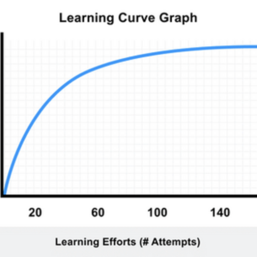
This concept is not unfamiliar to machine learning algorithms—to the contrary, most machine learning algorithms expressly dictate the number of data points sufficient to reach the plateau of the above learning curve. Accordingly, the threshold question that any judge should consider when evaluating the admissibility of machine-learning garnered evidence is whether the dataset met that optimal point.
Will that optimal dataset number always be accurate?
No.
Will the machine learning algorithm be immune from error once it reaches that point?
No.
Is it perfect?
No, but it does provide us with a minimum viable metric that courts can use to test the sufficiency of machine learning-based evidence, and that’s a good start.
More Articles